CNNに取って代わると言われている画像分析手法、ViT(Vision Transformer)の実装方法についてまとめます。ViTの内容については以下を参照してください。ざっくりとした理解ですが、BERTの画像分析版だと思っています。
画像認識の大革命。AI界で話題爆発中の「Vision Transformer」を解説! - Qiita
1. 実装方法について
以下はViTをファインチューニングする場合のソースコードです。Kaggleで公開されていたコードを参考にしています。本記事末尾にCIFAR10でファインチューニングしたときに使用したソースコードを載せますので、良ければそちらも見てください。
!pip install vit-keras

from tensorflow.keras.models import Sequential
from tensorflow.keras.layers import Dense, BatchNormalization, Flatten
from tensorflow.keras import optimizers
from vit_keras import vit, utils
import tensorflow_addons as tfa

image_size = 352

def buildModel():
    vit_model = vit.vit_b16(
        image_size = image_size,
        activation = 'sigmoid',
        pretrained = True,
        include_top = False,
        pretrained_top = False)
    model = tf.keras.Sequential([
        vit_model,
        tf.keras.layers.Flatten(),
        tf.keras.layers.BatchNormalization(),
        tf.keras.layers.Dense(11, activation = tfa.activations.gelu),
        tf.keras.layers.BatchNormalization(),
        tf.keras.layers.Dense(num_classes, 'softmax')
    ],
    name = 'vision_transformer')
    model.compile(optimizer=optimizers.Adam(learning_rate=1e-4), loss="categorical_crossentropy", metrics=["accuracy"])

    return model

model = buildModel()
2. ViTとして公開されているモデルの種類
公開されている主なモデルは以下の通りです。
- ViT-B_16
- ViT-B_32
- ViT-L_16
- ViT-L_32
上記のBとかLとかはモデルのサイズを表します。BはBase、LはLargeなので、大小関係はB<Lです。
16とか32はパッチサイズです。パッチとはViTに投入するために分割した画像のことです。16の場合は16×16のパッチをViTに投入することになります。
パッチについては以下のイメージでなんとなく伝わると思います。
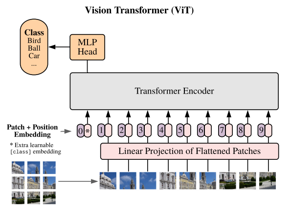
(参考:https://openreview.net/pdf?id=YicbFdNTTy)
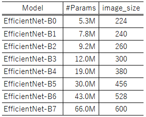
Largeよりも大きいHugeというモデルも存在するようですが、公開はされていないようです。ちなみに各モデルのパラメータ数は以下の通りとのことです。
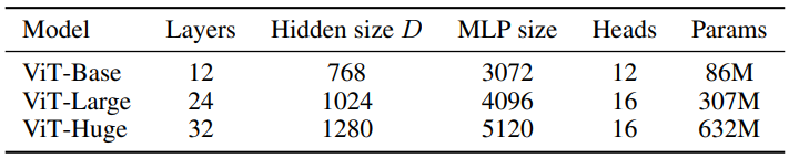
(参考:https://openreview.net/pdf?id=YicbFdNTTy)
3. 画像サイズについて
image_sizeはパッチサイズに依存し、パッチサイズの倍数である必要があるようです。ViT-B_16の場合、image_sizeとして224や240等を設定することが可能になります。
参考:ソースコード(CIFAR10でfine-tune)
import os
os.environ['PYTHONHASHSEED'] = '0'
import tensorflow as tf
os.environ['TF_DETERMINISTIC_OPS'] = 'true'
os.environ['TF_CUDNN_DETERMINISTIC'] = 'true'

import numpy as np
import random as rn

SEED = 123
def reset_random_seeds():
    tf.random.set_seed(SEED)
    np.random.seed(SEED)
    rn.seed(SEED)

reset_random_seeds()

session_conf = tf.compat.v1.ConfigProto(intra_op_parallelism_threads=32, inter_op_parallelism_threads=32)
tf.compat.v1.set_random_seed(SEED)
sess = tf.compat.v1.Session(graph=tf.compat.v1.get_default_graph(), config=session_conf)
import pandas as pd
import cv2
from tensorflow.keras.models import Sequential
from tensorflow.keras.layers import Dense, BatchNormalization,Flatten
from tensorflow.keras.utils import to_categorical
from tensorflow.keras.preprocessing.image import ImageDataGenerator
from tensorflow.keras import optimizers
from tensorflow.keras.callbacks import ReduceLROnPlateau, EarlyStopping
import tensorflow_addons as tfa
from vit_keras import vit, utils
from sklearn.model_selection import train_test_split
from tensorflow.keras.datasets import cifar10
(x_train, y_train), (x_test, y_test) = cifar10.load_data()
image_size = 128
input_shape=(image_size,image_size,3)
num_classes = 10
def upscale(image):
size = len(image)
data_upscaled = np.zeros((size, image_size, image_size, 3,))
for i in range(len(image)):
data_upscaled[i] = cv2.resize(image[i], dsize=(image_size, image_size), interpolation=cv2.INTER_CUBIC)
image = np.array(data_upscaled, dtype=np.int)
return image
x_train = upscale(x_train)
x_test = upscale(x_test)
def buildModel_ViT():
vit_model = vit.vit_b16(
image_size = image_size,
activation = 'sigmoid',
pretrained = True,
include_top = False,
pretrained_top = False)
model = tf.keras.Sequential([
vit_model,
tf.keras.layers.Flatten(),
tf.keras.layers.BatchNormalization(),
tf.keras.layers.Dense(21, activation = tfa.activations.gelu),
tf.keras.layers.BatchNormalization(),
tf.keras.layers.Dense(num_classes, 'softmax')
],
name = 'vision_transformer')
model.compile(optimizer=optimizers.Adam(learning_rate=1e-4), loss="categorical_crossentropy", metrics=["accuracy"])
return model
def train_vit_holdout(X, y, steps_per_epoch, epochs, batch_size, callbacks):
X_train, X_valid, y_train, y_valid = train_test_split(X, y, test_size=0.2, stratify=y, shuffle=True)
y_train = to_categorical(y_train)
y_valid = to_categorical(y_valid)
datagen = ImageDataGenerator(rotation_range=20, horizontal_flip=True, zoom_range=0.2)
train_generator = datagen.flow(X_train, y_train,batch_size=batch_size)
model = buildModel_ViT()
history = model.fit(train_generator,
steps_per_epoch=steps_per_epoch,
epochs=epochs,
validation_data=(X_valid, y_valid),
callbacks=callbacks,
shuffle=True
)
return model, history
batch_size = 32
steps_per_epoch = 1250
epochs = 1000
reduce_lr = ReduceLROnPlateau(monitor='val_accuracy',
factor=0.2,
patience=2,
verbose=1,
min_delta=1e-4,
min_lr=1e-6,
mode='max'
)
earlystopping = EarlyStopping(monitor='val_accuracy',
min_delta=1e-4,
patience=5,
mode='max',
verbose=1
)
callbacks = [earlystopping, reduce_lr]
model, history = train_vit_holdout(x_train, y_train, steps_per_epoch, epochs, batch_size, callbacks)
X = x_test
pred = model.predict(X)
df_pred = pd.DataFrame(pred)
pred = np.array(df_pred.idxmax(axis=1))
df_pred = pd.DataFrame(pred)
df_y = pd.DataFrame(y_test)
df_result = pd.concat([df_y, df_pred], axis=1, join_axes=[df_y.index])
df_result.columns = ['y','pred']
display(df_result)
from sklearn.metrics import accuracy_score, precision_score, recall_score, f1_score, confusion_matrix
print('Confusion Matrix:')
print(confusion_matrix(df_result['y'],df_result['pred']))
print()
print('Accuracy :{:.4f}'.format(accuracy_score(df_result['y'],df_result['pred'])))
print('Precision:{:.4f}'.format(precision_score(df_result['y'],df_result['pred'],average='macro')))
print('Recall :{:.4f}'.format(recall_score(df_result['y'],df_result['pred'],average='macro')))
print('F_score :{:.4f}'.format(f1_score(df_result['y'],df_result['pred'],average='macro')))